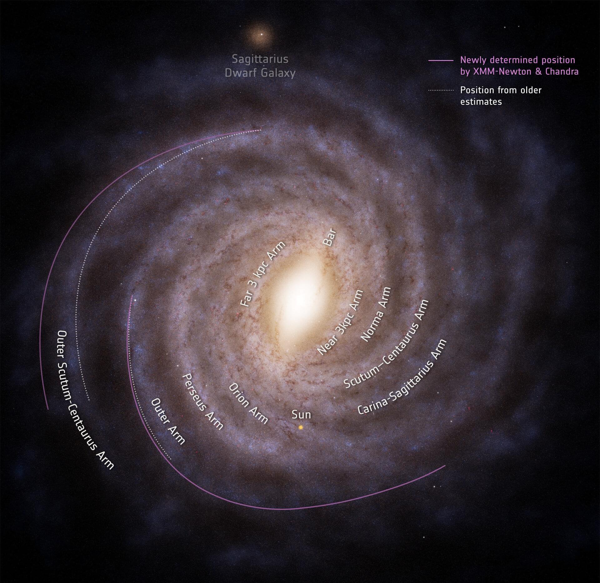
Toggle light / dark theme

Glaciers separate from the continental ice sheets in Greenland and Antarctica covered a global area of approximately 706,000 km2 around the year 200019, with an estimated total volume of 158,170 ± 41,030 km3, equivalent to a potential sea-level rise of 324 ± 84 mm (ref. 20). Glaciers are integral components of Earth’s climate and hydrologic system1. Hence, glacier monitoring is essential for understanding and assessing ongoing changes21,22, providing a basis for impact2,3,4,5,6,7,8,9,10 and modelling11,12,13 studies, and helping to track progress on limiting climate change23. The four main observation methods to derive glacier mass changes include glaciological measurements, digital elevation model (DEM) differencing, altimetry and gravimetry. Additional concepts include hybrid approaches that combine different observation methods. In situ glaciological measurements have been carried out at about 500 unevenly distributed glaciers24, representing less than 1% of Earth’s glaciers19. Glaciological time series provide seasonal-to-annual variability of glacier mass changes25. Although these are generally well correlated regionally, long-term trends of individual glaciers might not always be representative of a given region. Spaceborne observations complement in situ measurements, allowing for glacier monitoring at global scale over recent decades. Several optical and radar sensors allow the derivation of DEMs, which reflect the glacier surface topography. Repeat mapping and calculation of DEM differences provide multi-annual trends in elevation and volume changes26 for all glaciers in the world27. Similarly, laser and radar altimetry determine elevation changes along linear tracks, which can be extrapolated to calculate regional estimates of glacier elevation and volume change28. Unlike DEM differencing, altimetry provides spatially sparse observations but has a high (that is, monthly to annual) temporal resolution26. DEM differencing and altimetry require converting glacier volume to mass changes using density assumptions29. Satellite gravimetry estimates regional glacier mass changes at monthly resolution by measuring changes in Earth’s gravitational field after correcting for solid Earth and hydrological effects30,31. Although satellite gravimetry provides high temporal resolution and direct estimates of mass, it has a spatial resolution of a few hundred kilometres, which is several orders of magnitude lower than DEM differencing or altimetry26.

The heterogeneity of these observation methods in terms of spatial, temporal and observational characteristics, the diversity of approaches within a given method, and the lack of homogenization challenged past assessments of glacier mass changes. In the Intergovernmental Panel on Climate Change (IPCC)’s Sixth Assessment Report (AR6)16, for example, glacier mass changes for the period from 2000 to 2019 relied on DEM differencing from a limited number of global27 and regional studies16. Results from a combination of glaciological and DEM differencing25 as well as from gravimetry30 were used for comparison only. The report calculated regional estimates over a specific baseline period (2000–2019) and as mean mass-change rates based on selected studies per region, which only partly considered the strengths and limitations of the different observation methods.

The spread of reported results—many outside uncertainty margins—and recent updates from different observation methods afford an opportunity to assess regional and global glacier mass loss with a community-led effort. Within the Glacier Mass Balance Intercomparison Exercise (GlaMBIE; https://glambie.org), we collected, homogenized and combined regional results from the observation methods described above to yield a global assessment towards the upcoming IPCC reports of the seventh assessment cycle. At the same time, GlaMBIE provides insights into regional trends and interannual variabilities, quantifies the differences among observation methods, tracks observations within the range of projections, and delivers a refined observational baseline for future impact and modelling studies.

Head to https://squarespace.com/artem to save 10% off your first purchase of a website or domain using code ARTEMKIRSANOV

Socials:
X/Twitter: https://twitter.com/ArtemKRSV
Patreon: / artemkirsanov.

My name is Artem, I’m a graduate student at NYU Center for Neural Science and researcher at Flatiron Institute.

In this video video we are exploring a fascinating paper which revealed the role of biological constraints on what patterns of neural dynamics the brain and cannot learn.

Augmented reality (AR) has become a hot topic in the entertainment, fashion, and makeup industries. Though a few different technologies exist in these fields, dynamic facial projection mapping (DFPM) is among the most sophisticated and visually stunning ones. Briefly put, DFPM consists of projecting dynamic visuals onto a person’s face in real-time, using advanced facial tracking to ensure projections adapt seamlessly to movements and expressions.

While imagination should ideally be the only thing limiting what’s possible with DFPM in AR, this approach is held back by technical challenges. Projecting visuals onto a moving face implies that the DFPM system can detect the user’s facial features, such as the eyes, nose, and mouth, within less than a millisecond.

Even slight delays in processing or minuscule misalignments between the camera’s and projector’s image coordinates can result in projection errors—or “misalignment artifacts”—that viewers can notice, ruining the immersion.

“ tabindex=”0” accuracy and scale, brings scientists closer to understanding how neurons connect and communicate.

Mapping Thousands of Synaptic Connections

Harvard researchers have successfully mapped and cataloged over 70,000 synaptic connections from approximately 2,000 rat neurons. They achieved this using a silicon chip capable of detecting small but significant synaptic signals from a large number of neurons simultaneously.

Summary: Researchers have developed a geometric deep learning approach to uncover shared brain activity patterns across individuals. The method, called MARBLE, learns dynamic motifs from neural recordings and identifies common strategies used by different brains to solve the same task.

Tested on macaques and rats, MARBLE accurately decoded neural activity linked to movement and navigation, outperforming other machine learning methods. The system works by mapping neural data into high-dimensional geometric spaces, enabling pattern recognition across individuals and conditions.

MIT researchers developed a new approach for assessing predictions with a spatial dimension, like forecasting weather or mapping air pollution.

Re relying on a weather app to predict next week’s temperature. How do you know you can trust its forecast? Scientists use statistical and physical models to make predictions about everything from weather to air pollution. But checking whether these models are truly reliable is trickier than it seems—especially when the locations where we have validation data don Traditional validation methods struggle with this problem, failing to provide consistent accuracy in real-world scenarios. In this work, researchers introduce a new validation approach designed to improve trust in spatial predictions. They define a key requirement: as more validation data becomes available, the accuracy of the validation method should improve indefinitely. They show that existing methods don’t always meet this standard. Instead, they propose an approach inspired by previous work on handling differences in data distributions (known as “covariate shift”) but adapted for spatial prediction. Their method not only meets their strict validation requirement but also outperforms existing techniques in both simulations and real-world data.

By refining how we validate predictive models, this work helps ensure that critical forecasts—like air pollution levels or extreme weather events—can be trusted with greater confidence.


A new evaluation method assesses the accuracy of spatial prediction techniques, outperforming traditional methods. This could help scientists make better predictions in areas like weather forecasting, climate research, public health, and ecological management.

Astronomer Calvin Leung was excited last summer to crunch data from a newly commissioned radio telescope to precisely pinpoint the origin of repeated bursts of intense radio waves—so-called fast radio bursts (FRBs)—emanating from somewhere in the northern constellation Ursa Minor.

Leung, a Miller Postdoctoral Fellowship recipient at the University of California, Berkeley, hopes eventually to understand the origins of these mysterious bursts and use them as probes to trace the large-scale structure of the universe, a key to its origin and evolution. He had written most of the computer code that allowed him and his colleagues to combine data from several telescopes to triangulate the position of a burst to within a hair’s width at arm’s length.

The excitement turned to perplexity when his collaborators on the Canadian Hydrogen Intensity Mapping Experiment (CHIME) turned optical telescopes on the spot and discovered that the source was in the distant outskirts of a long-dead elliptical galaxy that by all rights should not contain the kind of star thought to produce these bursts.

To see how cognitive maps form in the brain, researchers used a Janelia-designed, high-resolution microscope with a large field of view to image neural activity in thousands of neurons in the hippocampus of a mouse as it learned. Credit: Sun and Winnubst et al.

Our brains build maps of the environment that help us understand the world around us, allowing us to think, recall, and plan. These maps not only help us to, say, find our room on the correct floor of a hotel, but they also help us figure out if we’ve gotten off the elevator on the wrong floor.

Neuroscientists know a lot about the activity of neurons that make up these maps – like which cells fire when we’re in a particular location. But how the brain creates these maps as we learn remains a mystery.

We explore numerically the complex dynamics of multilayer networks (consisting of three and one hundred layers) of cubic maps in the presence of noise-modulated interlayer coupling (multiplexing noise). The coupling strength is defined by independent discrete-time sources of color Gaussian noise. Uncoupled layers can demonstrate different complex structures, such as double-well chimeras, coherent and spatially incoherent regimes. Regions of partial synchronization of these structures are identified in the presence of multiplexing noise. We elucidate how synchronization of a three-layer network depends on the initially observed structures in the layers and construct synchronization regions in the plane of multiplexing noise parameters “noise spectrum width – noise intensity”

The default mode network (DMN) is a set of interconnected brain regions known to be most active when humans are awake but not engaged in physical activities, such as relaxing, resting or daydreaming. This brain network has been found to support a variety of mental functions, including introspection, memories of past experiences and the ability to understand others (i.e., social cognitions).

The DMN includes four main brain regions: the (mPFC), the (PCC), the angular gyrus and the hippocampus. While several studies have explored the function of this network, its anatomical structure and contribution to information processing are not fully understood.

Researchers at McGill University, Forschungszentrum Jülich and other institutes recently carried out a study aimed at better understanding the anatomy of the DMN, specifically examining the organization of neurons in the tissue of its connected brain regions, which is known as cytoarchitecture. Their findings, published in Nature Neuroscience, offer new indications that the DMN has a widespread influence on the human brain and its associated cognitive (i.e., mental) functions.